나이브 베이즈(Naive Bayes) 실습 with 데싸노트

나이브 베이즈는 베이즈 정리를 활용한 조건부 확률 기반의 분류 모델이다. 딥러닝만큼은 아니지만 간단한 방법으로 자연어처리를 원할 때 사용한다. 범용성이 높지는 않지만 독립변수들이 모두 독립적이라면 충분히 경쟁력 있는 모델이다. 딥러닝을 제외하고 자연어 처리에 가장 적합한 알고리즘이다. 속도도 빠르며, 작은 훈련 셋으로도 잘 예측한다. 

범주 형태의 변수가 많을 때 적합하고, 독립변수가 독립적일 경우 그 중요도가 비슷할 때 사용된다. 숫자형 변수가 많을 때는 적합하지 않다. 독립변수가 많을 때 상대적으로 더 작동하고, 독립변수의 상관관계가 없음을 전제로 한다.

문제 정의

스팸문자 여부를 판별해본다.

데이터 불러오기 및 확인 

import pandas as pd
import numpy as np
import matplotlib.pyplot as plt
import seaborn as sns

file_url = 'https://media.githubusercontent.com/media/musthave-ML10/data_source/main/spam.csv'
data = pd.read_csv(file_url)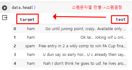

ham은 스팸이 아닌 문자, spam은 스팸인 문자를 뜻한다.

data['target'].unique()
# array(['ham', 'spam'], dtype=object)

전처리: 특수기호 제거, 불용어 제거, 목표형태 칼럼 변경하기, 카운트 기반으로 벡터화

특수기호 제거 

import string

def remove_punc(x):
    new_string = []
    for i in x:
        if i not in string.punctuation:
            new_string.append(i)
    new_string = ''.join(new_string)
    return new_string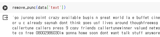

함수를 만들어서 특수기호를 제거해 보면 모든 문자열이 합쳐짐을 볼 수 있다. 따로따로 적용하기 위해서 

apply라는 함수를 적용해 주겠다.

data['text'] = data['text'].apply(remove_punc)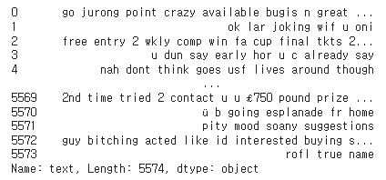

불용어 제거

import nltk #임포트
nltk.download('stopwords') #불용어 목록 가져오기
from nltk.corpus import stopwords #불용어 목록 임포트
stopwords.words('english') #영어 불용어 선택
print(stopwords.fileids()) #불용어 목록 확인

['arabic', 'azerbaijani', 'basque', 'bengali', 'catalan', 'chinese', 'danish', 'dutch', 'english', 'finnish', 'french', 'german', 'greek', 'hebrew', 'hinglish', 'hungarian', 'indonesian', 'italian', 'kazakh', 'nepali', 'norwegian', 'portuguese', 'romanian', 'russian', 'slovene', 'spanish', 'swedish', 'tajik', 'turkish']

def stop_words(x):
    new_string=[]
    for i in x.split():
        if i.lower() not in stopwords.words('english'):
            new_string.append(i.lower())
    new_string = ' '.join(new_string)
    return new_string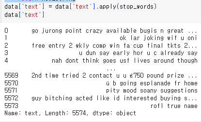

목표 칼럼 형태 변경

data['target'] = data['target'].map({'spam':1,'ham':0})

문자인 spam과 ham을 숫자로 변경 

카운트 기반 벡터화

모든 단어들을 사전처럼 모은 뒤 인덱스를 부여하고, 문장마다 속한 단어가 있는 인덱스를 카운트함 

x= data['text'] #독립변수	
y = data['target'] #종속변수

from sklearn.feature_extraction.text import CountVectorizer

cv = CountVectorizer() #객체 생성
cv.fit(x) #학습	
cv.vocabulary_ #단어와 인덱스 출력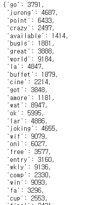

단어마다 인덱스가 되는 것을 볼 수 있다.

x= cv.transform(x)
print(x)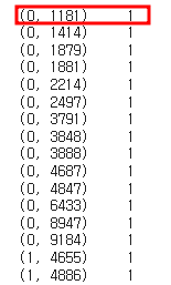

트랜폼 시킨 후 출력해 보면 좌부터 행, 인덱스, 출현 횟수를 나타내는 것을 확인할 수 있다.

from sklearn.model_selection import train_test_split
x_train, x_test, y_train, y_test = train_test_split(x,y,test_size=0.2, random_state=100)

독립변수/종속변수에 대한 훈련 셋/시험 셋 분할하기 

from sklearn.naive_bayes import MultinomialNB
model = MultinomialNB() #모델 객체 생성
model.fit(x_train, y_train) #학습
pred = model.predict(x_test) #예측

MultinomialNB는 나이브 베이즈 알고리즘으로 다항분호에 대한 알고리즘이다. 이외에도 Gaussian, Bernoulli 베르누이 분호에 따른 NB모듈이 있다. 

from sklearn.metrics import accuracy_score, confusion_matrix

accuracy_score(y_test,pred)
#0.9856502242152466

accuracy_score를 통해 정확도를 계산할 수 있다.

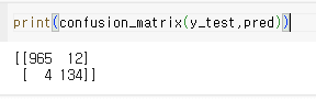
confusion matrix로도 확인할 수 있는데 

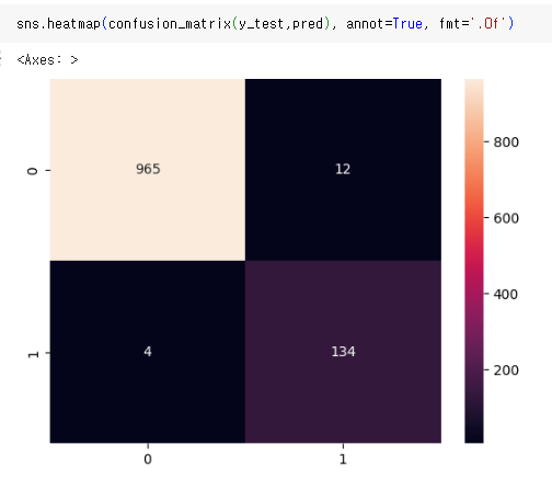
heatmap으로도 나타낼 수 있다. 

confusion matrix를 좀 더 알아보면 

True Negative(TN) 음성을 음성으로 판단	False Positive(FP) 음성을 양성으로 판단
False Negative(FN) 양성을 음성으로 판단	True Positive(TP) 양성을 양성으로 판단

따라서 이 실습에서는 (965+134)/(965+134+12+4) = 98%(약) 나오고, 이는 accuracy_score랑 동일하다. 

 

결과적으로 98%의 정확도로 스팸처리를 잘하는 것을 확인할 수 있다.